Basic Axioms, Bayes' Theorem & Interview Prep

A Practical Guide for Data Science, Part 1

In simple terms, probability is a framework that allows us to study uncertainty. Whether you’re a data scientist, or a machine learning researcher, you’ll deal with data, and a solid understanding of probability is indispensable. So here is what you can expect to learn in this part of the series:

• basic concepts of probability: events, experiments and outcomes

• axioms, rules and principles in probability

• some python simulations to deepen your understanding

• bonus: a couple questions you can expect to see in data science interviews

Let’s get started.

Events, experiments and outcomes

An event is just a possible outcome of the experiment. When you flip a coin, the event could be landing a heads up or a tails up. An experiment is a process that generates an outcome. For example, rolling a die, flipping a coin, measuring the temperature on a given day are all experiments because they all have multiple possible outcomes.

Now that we have those down, let’s do a simple coin flip simulation. Heads is 1, and tails is 0, and we can assume the coin is fair.

import random

def flip_coin():
  return random.choice([0,1])

Because we know the coin is fair, we know that if we flip the coin a 100 times, we can expect a roughly equal number of heads and tail ups.

def hundred_flips(n=100):
  result=[]
  for i in range(0,n):
    result.append(flip_coin())
  return result

flips=hundred_flips(n=100)
num_heads = sum(flips)
num_tails = len(flips) - num_heads

print(f"Number of Heads: {num_heads}") # 48
print(f"Number of Tails: {num_tails}") # 52

As you can see, we got 48 heads and 52 tails. We can expect to get similar numbers if we repeat this a thousand more times, and look at the distribution of heads ups.

import matplotlib.pyplot as plt

def run_experiment(num_flips=100, num_trials=1000):
  heads_counts=[]
  for _ in range(num_trials):
    flips = hundred_flips(num_flips)
    heads=sum(flips)
    heads_counts.append(heads)
  return heads_counts

heads_counts=run_experiment()

plt.hist(heads_counts, bins=range(30,70), alpha=0.75)
plt.title('Distribution of Heads in 100 Coin Flips')
plt.xlabel('Number of heads')
plt.ylabel('Frequency')
plt.show()

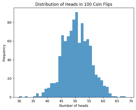
In the above simulation, we flip a coin 100 times as we did before, and repeat that a 1000 times, and in each trial keep track of the number of heads we get in each 100-flip sequence. When we plot this distribution, we see that the plot roughly simulates a normal distribution, which is what we expected.

Axioms, rules and principles

So now let’s talk about axioms, or the laws of probability.

1. Non-negative probability: This just means the probability of any event is at least 0, i.e. P(E)≥0,∀E∈Ω, and here E is the event and Ω is the sample space (i.e. for all events in sample space). Note that it can be 0, just has to be non-negative.

2. Certainty of sample space: The one means that something must happen. The total probability over the entire sample space is 1, i.e.:

   \(P(\Omega) = \sum_{E \in \Omega} P(E) = 1\)

3. Addition rule for mutually exclusive events: So if you have a mutually exclusive event, E_i​, it’s probability of occurring is the sum of it’s individual probabilities. A coin flip outcome can not be heads and tails at the same time, i.e. heads and tails are mutually exclusive. The probability of both, P(H⋃T) = P(H) + P(T). By extension:

   \(P\left(\bigcup_{i=1}^{\infty} E_i\right) = \sum_{i=1}^{\infty} P(E_i)\)

Conditional probability

For two events, A and B, conditional probability, P(A|B), is the probability that event A happens when one assumes that event B has already happened.

Let’s say we want to calculate P(A|B) for rolling a six-sided die. Event A is rolling an odd number and event B is rolling a number less than 3, i.e.:

Event A: {1, 3, 5}, Event B: {1, 2}

From basic probability we know:

• the theoretical probability of getting an odd number, P(A) =3/6 = 0.5

• the theoretical probability of getting a number <3, P(B) = 2/6 =0.33

• the theoretical probability of getting both, P(A∩B)=1/6 = 0.167 because only one number (1) satisfies both conditions.

• for conditional probability, P(A|B), we use formula P(A∩B)/P(B)=0.167/0.33=0.5

Let’s simulate this.

import random

# Event A: {1, 3, 5}
# Evnet B: {1, 2}

def simulate_die_rolls(num_rolls=100):
  count_A = 0
  count_B = 0
  count_A_and_B = 0

  for _ in range(num_rolls):
    roll = random.randint(1,6)
    is_A = roll in [1, 3, 5]
    is_B = roll in [1, 2]
    if is_A:
      count_A+=1
    if is_B:
      count_B+=1
    if is_A and is_B:
      count_A_and_B +=1

  p_A = count_A / num_rolls
  p_B = count_B / num_rolls
  p_A_and_B = count_A_and_B / num_rolls

  p_A_given_B = count_A_and_B / count_B

  is_independent = p_A_and_B == (p_A * p_B)

  return p_A, p_B,  p_A_and_B, p_A_given_B, is_independent

p_A, p_B, p_A_and_B, p_A_given_B, is_independent=simulate_die_rolls(num_rolls=10000)

print(f"P(A) = {p_A}")
print(f"P(B) = {p_B}")
print(f"P(A and B) = {p_A_and_B}")
print(f"P(A|B) = {p_A_given_B}")
print(f"Are A and B independent? {is_independent}")

Result:

P(A) = 0.4998
P(B) = 0.3342
P(A and B) = 0.163
P(A|B) = 0.48773189706762415
Are A and B independent? False

The simulated probabilities are close, which is a good sanity check. The P(A|B) value suggests that the if we know event B has occurred, there is a ~49% chance that event B will also occur. The independence check tells us that A and B are not independent, which makes sense. The more simulations you run, the closer you will get to the theoretical values we computed earlier.

Bayes’ rule

Bayes’ rule is a powerful tool for revising existing predictions or hypothesis given new evidence. You may have seen it in the context of medical diagnosis, spam filtering and other decision-making scenarios where you have some data and you want to make an informed decision. Here is how it is generally applied:

• P(A), prior probability: this is what you already know about event A happening without new evidence on event B

• P(B|A), likelihood: this tells you how likely B is assuming A is true

• P(B), marginal likelihood: this tells you how likely new evidence B is under all possible values of A

• P(A|B), posterior probability: this (goal of Bayes’ theorem) tells you how likely A is given some new evidence B

The general formula for Bayes’ rule is:

P(B|A) = (P(B|A)P(A)) / P(B)

Say, for example, we have a rare disease that affects 1% of the population. We also have to test for this disease that has a 95% true positive rate (TPR) and a 5% FPR. We want to know: if you get a positive test, what is the chance you actually have the disease?

P(disease | positive test) = P(positive test | disease) * P(disease) / P(positive test)

expanding P(positive test) = [ P(positive test | disease ) * P(disease) + P(positive test | no disease) * P(no disease)]

so, P(disease | positive test) = P(positive test | disease) * P(disease) / [ P(positive test | disease ) * P(disease) + P(positive test | no disease) * P(no disease)]

def bayes_rule(prior, tpr, fpr):

  # prior
  p_disease = prior # P(disease)

  # complement
  p_no_disease = 1-prior # P(no disease)

  # likelihood
  p_pos_given_disease = tpr # P(pos | disease)

  # fpr
  p_pos_given_no_disease = fpr # P(pos | no disease)

  #marginal
  p_pos = (p_disease * p_pos_given_disease) + (p_no_disease * p_pos_given_no_disease)

  #posterior
  p_disease_given_pos = (p_pos_given_disease * p_disease) / p_pos

  return p_disease_given_pos

prior=0.01
tpr=0.95
fpr=1-tpr

result = bayes_rule(prior, tpr, fpr)
print(result)

# 0.1610

So this implies that even though the test is 95% accurate, the chance of actually having the disease after testing is only about 16.10%. This is why Bayes’ theorem is so important. It includes prior probability into the calculation.

Combinatorics

Combinatorics is the study of counting things. There are two main ways of counting. Consider 3 apples, A_1, A_2, and A_3, and you’re picking 2 out of them. Two considerations:

• ordered vs. unordered: does the order matter? i.e. (A_1, A_2) different from (A_2, A_1)? if so, the selection process is ordered, otherwise unordered.

• with or without replacement: when selecting one object, is that object removed from future selection? if so, the selection process is said to have replacement.

Let's map some of these concepts to code.

• Ordered selection with replacement

For ordered selection with replacement, we have n^k possible selections :

def ordered_with_replacement(n,k):
  return n**k

n=3 # 3 apples
k=2 # pick 2
result =ordered_with_replacement(n,k)
print(result) # 9

(1,1), (1,2), (1,3), (2,1), (2,2), (2,3), (3,1), (3,2), (3,3)

For 3 apples, picking 2, we compute 3^2 = 9

• Ordered selection without replacement

For ordered selection without replacement, use n!/(n-k)!

from math import factorial

def ordered_without_replacement(n, k):
    return factorial(n) // factorial(n - k)

result = ordered_without_replacement(n, k)
print(result) # 6

(1,2), (1,3), (2,1), (2,3), (3,1), (3,2)

We compute 3!/(3-2)! = 6

• Unordered selection without replacement

For unordered selection without replacement, we use n!/(k! * (n-k)!)

def unordered_without_replacement(n, k):
    return factorial(n) // (factorial(k) * factorial(n - k))

result = unordered_without_replacement(n, k)
print(result) # 3

(1,2), (1,3), (2,3)

We compute 3!/(2!*(3-2)!)=3

• Unordered selection with replacement

For unordered selection with replacement, we use (n+k-1)!/k!(n-1)!

def unordered_with_replacement(n, k):
    return factorial(n + k - 1) // (factorial(k) * factorial(n - 1))

result = unordered_with_replacement(n, k)
print(result)

(1,1), (1,2), (1,3), (2,2), (2,3), (3,3)

We compute (3+2-1)!/(2!(3-1)!)=6

In each case, the results match up with the theoretical expectations, and we’ve also enumerated the sets of all possible selections.

Bonus: questions

1. Three zebras (E):

Three zebras are chilling in the desert. Suddenly a lion attacks.

Each zebra is sitting on a corner of an equally length triangle. Each zebra randomly picks a direction and only runs along the outline of the triangle to either edge of the triangle.

What is the probability that none of the zebras collide?

So each zebra can either run in a CW, or CCW direction.

P(CW) = P(CCW) = 1/2 * 1/2 * 1/2 = 1/8

so P(same direction) = P(CW) + P(CCW) = 1/4

2. Lazy Rater (E):

Netflix has hired people to rate movies.

Out of all of the raters, 80% of the raters carefully rate movies and rate 60% of the movies as good and 40% as bad. The other 20% are lazy raters and rate 100% of the movies as good.

Assuming all raters rate the same amount of movies, what is the probability that a movie is rated good?

P(careful) = 0.8

• P(rated good|careful) = 0.6

• P(rated bad|careful) = 0.4

P(lazy) = 0.2

• P(rated good|lazy) = 1.0

• P(rated bad|lazy) = 0

P(rated good)= P(rated good|careful)*P(careful) + P(rated good|lazy)*P(lazy) = 0.4*0.8 + 0.2*1=0.68

3. Fake Algorithm Reviews (E):

Let’s say we’re trying to determine fake reviews on our products. 

Based on past data, 98% reviews are legitimate and 2% are fake. If a review is fake, there is 95% chance that the machine learning algorithm identifies it as fake. If a review is legitimate, there is a 90% chance that the machine learning algorithm identifies it as legitimate.

What is the percentage chance the review is actually fake when the algorithm detects it as fake?

P(legit) = .98

P(fake) = .02

P(identified fake|fake) = 0.95 =

P(identified legit|legit) = 0.90

P(fake|identified fake) = ?

This is a Bayes’ theorem problem.

P(fake|identified fake) = P(identified fake|fake) P(fake)/P(identified fake)

P(identified fake) = P(identified fake|fake) P(fake) + P(identified fake|legit) P(legit)

P(fake|identified fake) = 0.95 * 0.02 / [(0.95*0.2) + ((1-0.90)+0.98)]

= 0.162

---

That’s all for now! ✌🏼In the next part, we will talk about discrete distributions.